Choosing the right quantum error reduction strategy: A practical guide to error suppression, error mitigation, and quantum error correction

Quantum computers hold transformative promise, with applications in finance, AI, chemistry, logistics, and transportation all set to be radically disrupted by the emergence of new quantum-powered solutions. Development is accelerating—leading providers (IBM, IonQ, and Oxford Quantum Circuits) are projecting large-scale devices delivering quantum advantage by the end of this decade.
Yet despite exceptional progress, today’s hardware remains limited by high error rates. Tackling these errors is the central challenge of the field; without effective reduction strategies, even the most advanced machines deliver unreliable results.
With all of the excitement about recent Quantum Error Correction (QEC) demonstrations it might seem the problem is solved—QEC is here to save the day and errors are a thing of the past.
Unfortunately, not quite. In practice, you cannot execute a fully error-corrected algorithm on any hardware available now or in the near future; you can only implement pieces of QEC, meaning the utility delivered for your application may be limited. And in most cases, QEC makes the overall processor worse. So how can you attack the problem of managing errors to increase the value of your quantum computing investment today?
Software-based techniques that suppress or mitigate errors are essential to unlocking near-term value and paving the way to quantum advantage. So, which to choose? There is a complex interplay between the mechanics of error-reduction techniques and the characteristics of a specific application, making the selection of the best strategy for handling errors a complex and challenging task.
We previously wrote about the basic differences between the core techniques to address errors: error suppression, error mitigation, and quantum error correction.
Here we provide a practical guide empowering you to understand how and when to select between these methods when executing your target quantum applications. We also include a comprehensive appendix covering a wide variety of applications so you can simply look up a recommendation for the TL;DR.
Know your application first
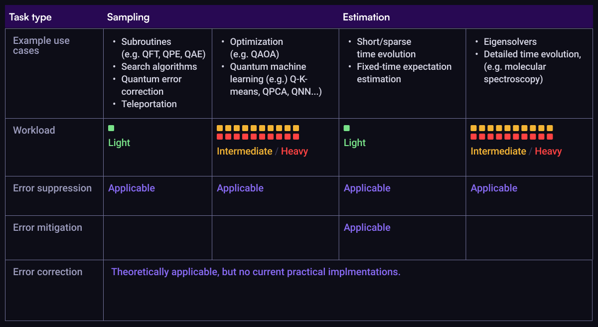
The first step in choosing a strategy comes from understanding the key characteristics of your use case. Not all algorithms have the same structures or characteristics, and their variability against a few key metrics determines which error-reduction strategies will work best for a given use case.
Output type, workload size, and circuit characteristics are the key things to consider when selecting error-reduction strategies. We go through these in detail below.
Output type: full distribution or average only
Quantum tasks generally fall into two output categories: sampling and estimation. We will see below that because the outputs differ so wildly between these categories, some error-management strategies are fully incompatible with certain applications.
Sampling tasks can provide a range of viable outputs (over different measured bitstrings), all of which are valid “answers” to the algorithmic query. The constituents and shape of this distribution contain critical information that must be preserved. By contrast, estimation tasks simply seek only the average value of some measurable parameter.
We can categorize many well-known algorithms against these types of output:
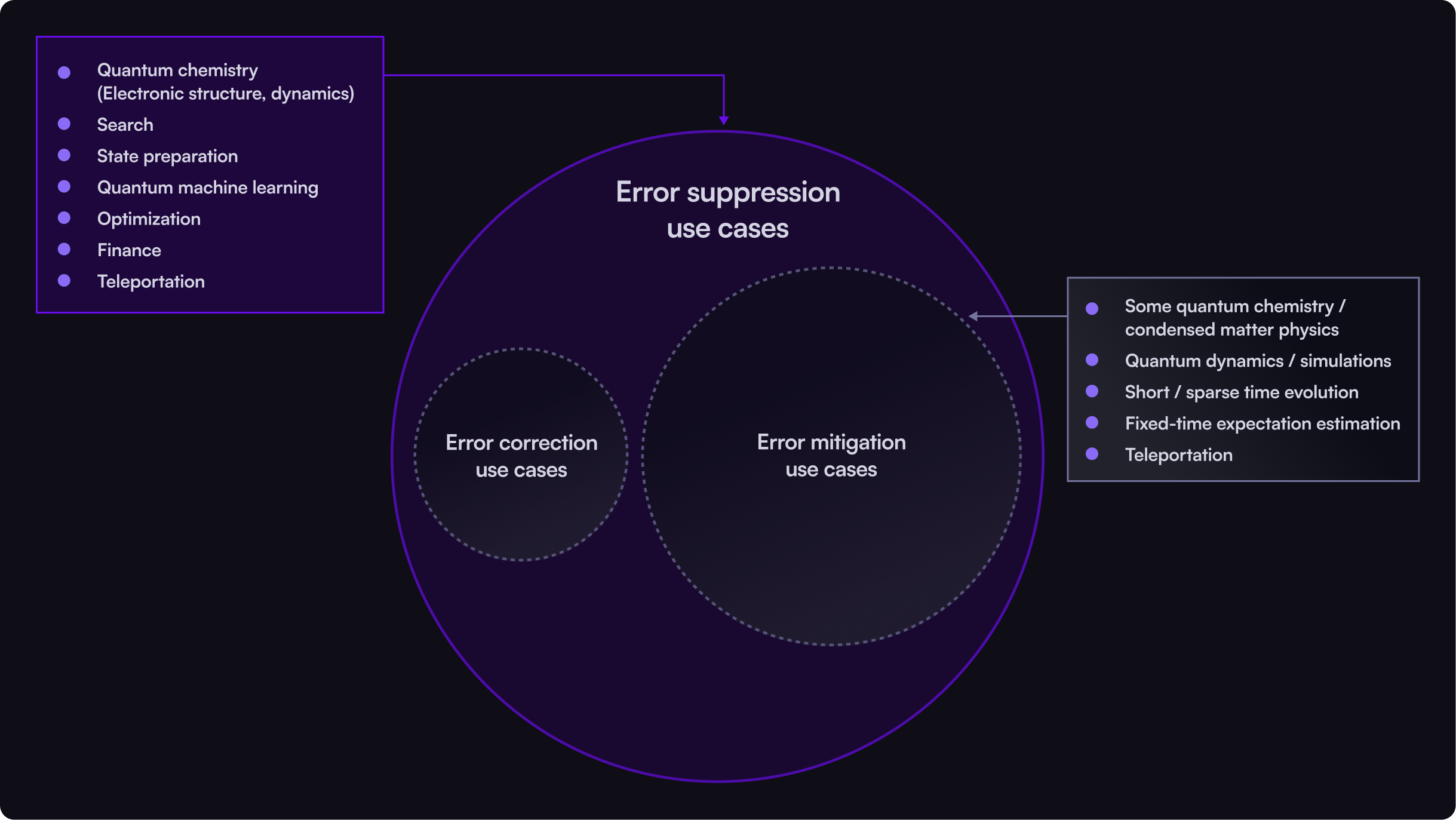
- Sampling tasks (bitstring probabilities): generate measurement outcomes in the form of bitstrings whose frequencies approximate an output probability distribution within the quantum state produced by a quantum circuit or process. For example, sampling-based algorithms (like SQD or Quantum Monte Carlo), optimization tasks such as QAOA, and most future quantum algorithms and subroutines (like Grover, QFT, QPE, and eventually QEC).
- Estimation tasks (expectation values): compute statistical properties of a quantum system—such as an observable’s mean value—based on repeated measurements of that system. For example, tasks common in quantum chemistry and condensed matter physics, variational algorithms, and simulations that rely on precise estimation of observables.
Workload sizes and shot counts
Most quantum applications do not involve a single execution of just one circuit representing the problem of interest. Quantum tasks can vary significantly in scale, from single circuits to workloads involving hundreds or thousands of circuit executions. The number of circuits and number of shots-per-circuit-execution (samples) directly impact the amount of computational overhead and overall execution time required for an application. Between these, the circuit count dominates execution time unless an extreme number of shots is required.
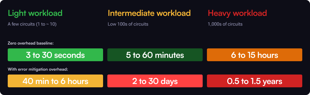
Workload sizes can roughly be characterized as follows:
- Light: fewer than 10 circuits,
- Intermediate: low 100s of circuits,
- Heavy: 1,000s of circuits.
These characteristics matter because, as we’ll see below, the overhead included in different error-reduction strategies can vary by orders of magnitude. A light task might handle some additional overhead well, but a heavy workload can be rendered totally impractical with the wrong error-reduction strategy.
Circuit width and depth
Even at the level of individual circuits, quantum applications span a broad range of characteristics.
As an example, circuits representing the time evolution of molecules and spin models can vary dramatically: simulating 3 time points of a 10-spin model on a line, for instance, requires 10 qubits and a circuit with a 2-qubit gate depth of only 3, whereas simulating the detailed dynamics of large molecules (like iron-clusters) requires a ~100 qubit circuit with 2-qubit gate depth of many 1000s.
When required circuit widths are high, preserving available data qubits will be a high priority. For error-reduction strategies that involve physical redundancy, this might prove a steep penalty, leaving insufficient qubit resources for the execution of the core algorithms.
For very deep circuits, users will typically face limits imposed by incoherent errors (so-called coherence limits). Since not all approaches to error management handle these errors equally, circuit depth may motivate selection of certain techniques over others.
Understand the limits of different error management strategies
Error suppression: A critical first line of defense for dominant errors
Error suppression corresponds to leveraging flexibility in quantum platform programming in order to execute a circuit correctly given anticipated imperfections in the hardware.
It proactively reduces the impact of noise at both the gate and circuit levels by either avoiding errors (e.g. via circuit routing or choice of gate set) or actively suppressing them via the physics of coherent averaging and dynamical decoupling in gate and circuit design. This technology is deterministic, meaning it provides effective error reduction in a single execution without the need for repeated execution or statistical averaging.
Error suppression is an effective first-line of defense for any application with any output characteristics. It can generally dramatically suppress coherent errors, but is unable to address incoherent errors exhibiting true randomness such as so-called T1 processes (AKA qubit incoherent lifetimes).
You can read more about the underlying technology and its construction in this technical manuscript.
Error mitigation: Improvement comes at exponential runtime cost
Error mitigation addresses noise in post-processing by averaging out the impact of noise that occurs during circuit execution. Unlike error suppression, it does not prevent errors, but rather reduces the average impact of the noise on the output, as determined by performing many repetitions of the target circuit and post-processing the outputs.
Commonly used methods include zero-noise extrapolation (ZNE) and probabilistic error cancellation (PEC). Both techniques are popular, and come with complementary tradeoffs: PEC provides a theoretical guarantee on the accuracy of solutions, at the cost of exponential overhead in preliminary device characterization, repeated circuit executions, and classical post-processing. On the other hand, ZNE obviates the need for exponential overhead, but in exchange omits performance guarantees. From here on, as we discuss these methods, we will keep PEC (and its closely related variants) in mind as it has gained considerable attention in recent times.
Error mitigation methods have the benefit that they can compensate for both coherent and incoherent error processes.
This comes with two very significant limitations. First they are not universally applicable. Importantly, they are not applicable when analyzing full output distributions of quantum circuits. This is a common requirement in most sampling algorithms, including some of the most important subroutines in the field. Second, the exponential overhead of most error mitigation methods applies a runtime performance penalty that can rapidly blow out to impractically long times.
These significant limits have largely constrained error mitigation routines to be deployed in the context of the simulation of physical and chemical systems, with limited relevance to other applications.
Quantum Error Correction: Powerful in principle, yet resource-intensive
Quantum error correction (QEC) is an algorithm designed to deliver error resilience via the addition of physical redundancy. Spreading quantum information across many qubits through the process of encoding provides a mechanism by which errors can be identified and corrected on a rolling basis as they occur.
This technique is foundational to quantum information theory. It showed that even though information in quantum systems is continuous, errors can be made discrete when using QEC. This simple observation is fundamental to the notion that it is even possible to build arbitrarily large quantum computers.
In general, QEC codes can be designed to handle any form of quantum error (even including qubit loss), and any arbitrary algorithm can be crafted to execute on encoded logical qubits rather than bare physical qubits. Many algorithms require so many qubits and operations that only QEC can feasibly deliver the necessary effective error rates.
This universality comes at a tremendous cost which limits utility today and will continue to limit utility for years to come.
First, QEC doesn’t “end” the existence of errors—it reduces their likelihood. The physical overhead rates required to suitably implement QEC and hit a target (reduced) error rate then depend on the selected code and the starting error rates. Unfortunately, in many extrapolations this ratio can be 1000:1 or more. Considering no one has yet operated a 1000 qubit quantum computer, this can be a significant penalty on today’s machines. For example, the recent Google demonstration with distance 7 surface code used a full device of 105 physical qubits to realize a single logical qubit. That is, even if things were working perfectly with their QEC demonstration, they’d only have one useful qubit—far too small to run any workload at all.
In addition, fault-tolerant execution (specifically, execution using QEC strategies that mathematically guarantee certain error-scaling properties) often runs thousands to millions of times slower than uncorrected circuits, severely restricting the feasibility of large-scale quantum computations. This of course comes from the error identification and correction process which must be executed, but also from the complexity in manipulating encoded logical qubits. Most codes don’t permit 1:1 operations between the constituents of two logical qubits in order to implement the same target operation (a property known as transversality). Accordingly, many additional operations are required in actual implementation, constituting a physical and timing overhead in logical-circuit execution.
In almost all demonstrations to date, even when logical-qubit error rates get lower than the bare physical-qubit values using QEC (a very hard threshold to achieve), the overall processor performance decreases due to these various forms of QEC overhead. The device will either be effectively much smaller or much slower to the point of greatly diminished utility.
More importantly, a comprehensive validated toolkit of QEC operations has yet to be fully demonstrated. Current demonstrations serve primarily as proof-of-concept rather than scalable solutions. Practical QEC use remains constrained to small-scale experiments until quantum hardware advances significantly, especially given the numbers of qubits needed to achieve Quantum Advantage.
Matching strategies to your quantum workloads
Now that you understand the critical characteristics of both your applications and the potential error reduction strategies available, it’s time to align these two sets of constraints.To help with this, we’ve made a quick summary that helps illustrate the key choices from a practical view, and we provide a comprehensive table in the appendix.
To suppress or to mitigate on today’s machines?
First, QEC is largely only used for scientific demonstrations on machines available today. Running algorithms using logically encoded qubits will remain less effective than alternate strategies until machines become much bigger. Otherwise if your workload requires QEC, you’ll have to wait for machines to get significantly larger. For a deeper dive on this issue, read more here.
So for workloads accessible on today’s machines you only need to choose whether to implement error suppression or error mitigation. Above we outline which classes of problem are compatible with error mitigation; now we’ll focus our discussion on problem scale when considering estimation tasks.
In execution, error suppression primarily introduces timing overhead during classical pre-processing phases like circuit compilation. This pre-processing typically adds only seconds or minutes to total execution time regardless of workload scale. Once compiled, circuits run natively on hardware, with minimal additional quantum runtime overhead. For workloads involving 100s to 1,000s of circuits, error suppression keeps total quantum execution times essentially unchanged—ranging from seconds or minutes for small tasks to only a few hours for the largest workloads.
For light workloads, error-mitigation overhead is manageable and the technique can yield precise results, especially when incoherent errors are problematic. However, for intermediate to large workloads, the exponential quantum-execution overhead of error mitigation quickly becomes impractical. For workloads involving 100s to 1,000s of circuits (typical for quantum optimization or machine learning) mitigation overhead can extend quantum runtimes from a few hours to weeks or months.
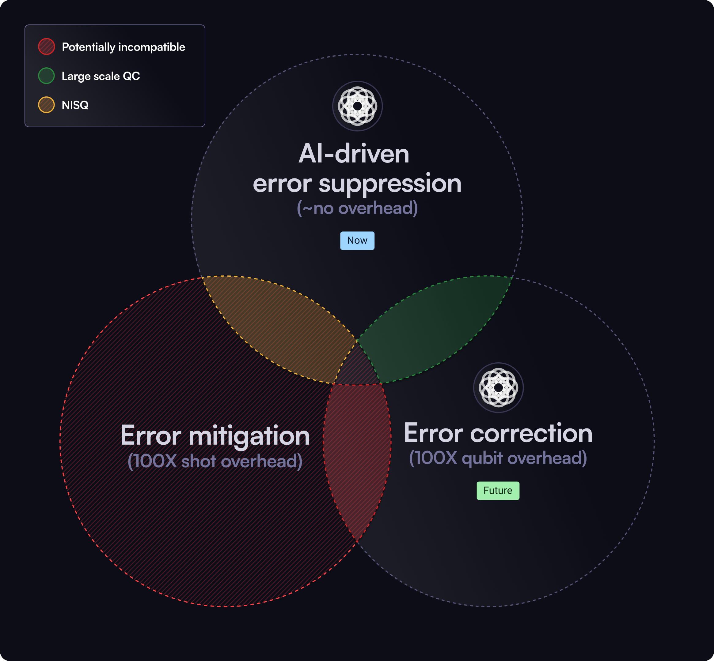
Strategic compatibility: Combining methods effectively
Quantum developers can maximize outcomes by strategically combining error-reduction strategies in ways that bring together complementary strengths:
- ✅ Suppression + mitigation: Suppression reduces the baseline impact of noise, thereby making mitigation more effective and less resource-intensive, and ensuring all classes of errors are efficiently reduced. This can be a potent combination in the NISQ era.
- ✅ Suppression + QEC: Lowering physical error rates through suppression can significantly ease QEC’s stringent resource demands. Doing so also therefore enables the maximization of performance on existing hardware, such as by improving the quality of QEC primitives. We see this as a key pathway for the future in large-scale quantum computing, and one already validated on real hardware.
- ❌ Mitigation + QEC: As QEC is a runtime method and mitigation is a post-processing-based method, they are not trivially compatible. Recent research suggests that implementing error mitigation after QEC at the logical level is theoretically possible, though there is not yet a consistent paradigm for characterizing noise models and performing mitigation at the logical level. More unfortunate still, this combination would multiply two sources of exponential overhead–one in time and one in qubits—potentially erasing even exponential scaling gains coming from the use of a quantum computer and making it unlikely that this combination will ever be practical for large-scale computing.
Strategically using these methods together (or not) ensures optimal performance on current hardware and prepares for future advancements.
Conclusion: A balanced, strategic path forward
Effectively managing quantum errors necessitates clarity on when and how to apply suppression, mitigation, and correction. Whether performing precise spectroscopy for quantum chemistry, extracting expectation values in variational algorithms, or scaling quantum optimization workloads, tailoring error-reduction strategies significantly impacts practical outcomes. So here are our key takeaway recommendations:
- Always implement error suppression: Implement suppression universally across all quantum tasks to ensure maximum baseline performance.
- Selectively apply mitigation, combined with error suppression: When workload size remains manageable and requires the estimation of high-accuracy expectation values, error mitigation can complement error suppression in achieving better estimation with relatively moderate overhead.
- Prepare for the arrival of practical QEC in the long term: Continue tracking the development and advancement of QEC technologies, maintaining realistic expectations regarding their near-term practical constraints.
As we look ahead we’re also excited by the prospect of new high-efficiency partial-QEC strategies that can deliver much higher value in the near term. For instance, recent demonstrations that combining gate-level optimization with bosonic encoding could get superconducting devices beyond breakeven, or that leveraging QEC primitives like error detection without full encoding could provide net improvements in device performance - including enabling a record rigorously benchmarked 75-qubit GHZ state—show that truly hybrid approaches may be the most promising pathway forward.
By taking a balanced, strategic approach—anchored by universally applicable error suppression, augmented selectively by mitigation, and preparing strategically for quantum error correction—quantum developers can optimize today's quantum hardware while paving the way for future quantum advancements.