Optimize hybrid quantum-classical algorithms directly with Fire Opal

Hybrid quantum-classical computing combines the best properties of both quantum and classical processors. By farming out a small but computationally challenging part of your problem to a quantum processing unit (QPU), you’re able to gain advantages while recognizing that quantum computers simply aren’t efficient at many tasks, like basic arithmetic.

The Quantum Approximate Optimization Algorithm (QAOA) is a popular hybrid quantum-classical algorithm applicable to a wide range of optimization problems that are out of reach today for enterprises, like financial portfolio optimization, efficient logistics routing, and asset-liability management.

We’re thrilled to announce a completely new capability available in Fire Opal: an end-to-end managed tool for high-performance hardware execution of QAOA. With this new feature, all aspects of running QAOA on real hardware are fully optimized to reduce errors and improve the quality of solutions—all with zero configuration on your part!

This is truly the only software in the entire industry focused on making the execution of QAOA useful on real hardware for all of your applications.

Implementing QAOA algorithms - it’s complicated

QAOA uses classical optimization techniques (executed on conventional CPUs), to iteratively update quantum circuits (executed on QPUs). This iterative process is the core idea behind most machine learning algorithms, like the training of a neural network. And it’s not much different from the way our team uses machine learning methods to optimize quantum logic gates, except the tunable parameters define a quantum circuit rather than an individual physical operation.

Implementing a QAOA algorithm with the expectation of getting useful results is complicated. Once you've set up the problem, there is still a complex configuration process you need to complete that requires a deep understanding of both conventional optimization and physics.

Then when you run it on a device, you'll rarely get an answer better than random selection. Even with the many implementations of QAOA on the market, an open secret within the industry is that it's very difficult to get meaningful results running QAOA on real hardware.

Fire Opal’s new QAOA solver alleviates the complexity and challenge of running these algorithms by providing an easy-to-use function that consistently returns the correct answer. It’s validated to enable the full QAOA implementation on hardware at a groundbreaking scale.

See the light in the dark with Fire Opal’s QAOA Solver

Fire Opal allows you to gain true insights from your quantum algorithms. It’s an out-of-the-box solution that automatically reduces error and boosts algorithmic success on quantum computers. It connects directly to supported hardware backends and returns the best output achievable without any user intervention, hardware knowledge, or configuration required.

Countless users have achieved useful results from devices that otherwise generate pure noise with Fire Opal.

“I thought Grover's algorithm was still far away in the scope of fault-tolerant quantum computing. I was surprised to find it is feasible already today, yet still on a small scale, with the help of Fire Opal.”

Ohad Lev, independent algorithm developer and researcher

Fire Opal delivers extraordinary results through error suppression in a single step with no configuration or settings; .execute takes care of everything for you.

Enjoy the simplicity of full QAOA execution in a single step

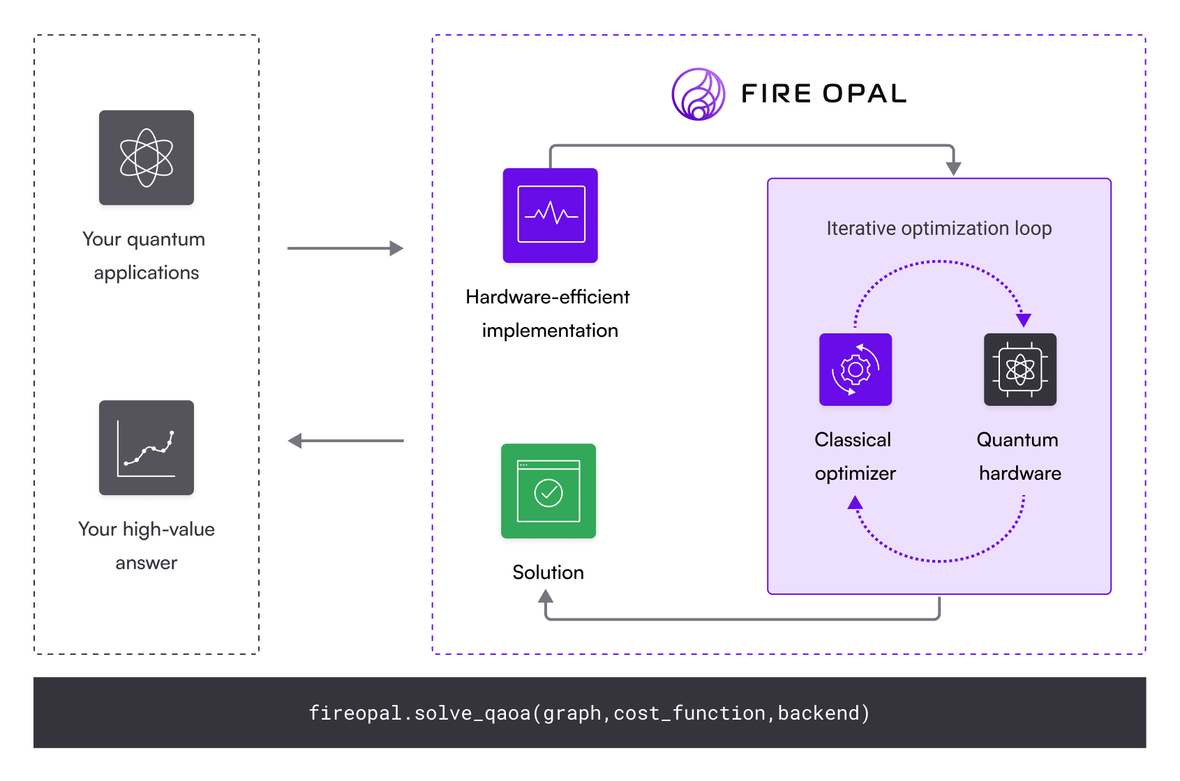
Simplicity is a core philosophy of Fire Opal. Similar to the .execute function that applies error suppression and runs your circuit with a single line of code, the new QAOA function handles all aspects of QAOA with just a single call: solve_qaoa.

You don’t need the expert knowledge typically required to build an implementation, apply the correct error-suppression and pulse-level programming techniques, or even build a reliable and high-performance classical “optimization loop”.

All you need to do is define the problem—you can simply input either a graph and a goal, or a cost function, and Fire Opal does the rest for you.

Test it out yourself by running our tutorial.

Get the right answer

Existing implementations of QAOA in many frameworks and software development kits (SDKs) return random outputs when executed on real hardware by either converging on the wrong answer or never reaching a solution at all. SDKs are convenient, but there’s a huge, unappreciated gap when it comes to achieving results on real quantum computers.

The new Fire Opal QAOA solver consistently returns the correct solution to the entire QAOA algorithm. We compared its performance to an open-source QAOA method, which we’ll refer to as the “default”. In ten repeated trials of a MaxCut problem, Fire Opal converged on the correct solution every time, whereas the default never produced a correct answer.

How does that happen?

The power of Fire Opal’s QAOA solver starts with improving the execution of every quantum circuit in the iterative procedure and extends through to the specific implementation of the classical loop that drives QAOA to find a solution.

Hybrid quantum algorithms are probabilistic, meaning there is a chance they will give the right solution. The aim when improving them is to boost the chance of returning the right solution. Figure 2 shows plots of the probability of the quantum computer outputting a “bitstring” that corresponds to a candidate solution to a problem. The ideal plot of probabilities is shown in the top graph, where we have highlighted the solution with the highest probability and noted in the legend the total probability of getting a valid solution. There can be multiple bitstrings that give the right answer, as is true in this case. Because the algorithm is probabilistic, even when everything works perfectly this total probability is less than 100%.

The bottom graph Figure 2 transitions between the results obtained from the default benchmark and those obtained using Fire Opal. You can see from the plots that when you run QAOA with the default benchmark, the probabilities of all the bitstrings are the same! It’s become a completely random choice of output. The probability of the best solution, in particular, is much smaller now and the QAOA algorithm isn’t delivering useful outputs.

In contrast, the Fire Opal boosted performance looks almost the same as the ideal plot. The top solution bitstring now has the highest probability, and the total probability of getting the right answer has increased by a factor of 12x.

When you run the QAOA algorithm with Fire Opal, the correct bitstring gets output with higher probability, meaning you can determine the right bistring in fewer iterations, which ultimately saves you QPU time.

The quality of QAOA circuit executions can also be illustrated by measuring the so-called “cost landscape”—the parameter space over which the classical part of the algorithm tries to find a minimum value. To visualize how this works, you can think of how water gradually makes its way to the lowest point on an uneven landscape with hills and valleys—QAOA more or less applies an algorithm to try to find that low point by measuring the “quantum landscape.”

Comparing the measured reconstruction of the landscape to the ideal simulated landscape is a great way to evaluate the quality of the QAOA algorithm’s implementation on hardware; if the landscapes are similar, that means the hardware returns results close to what’s expected under perfect conditions. If they’re very different, that means something has gone wrong in the hardware.

You can see just this comparison in the Figure 3 below. Simply stated, the default landscape looks nothing like the ideal picture of the simulation. It would be impossible to find the low point in this landscape since it’s largely random. By contrast the Q-CTRL picture looks almost identical to the ideal and has its target solution (the low point of the landscape) in the same place!

More specifically, Fire Opal’s QAOA solver demonstrated 200x improvement in reconstructing the ideal QAOA cost landscape using a metric called structural similarity (SSIM).

This update is almost an order of magnitude better than previous, already significant, demonstrations published in our benchmarking results!

Save time and compute resources

Running hybrid algorithms can be resource-intensive, requiring numerous iterations, or steps in the optimization loop to perform a single trial. As quantum compute time is becoming a relatively expensive resource, everyone is becoming more mindful of how efficiently they can implement algorithms.

Failed QAOA execution on hardware wastes compute time and expenditure—hundreds or even thousands of dollars thrown out the window with no useful insights to show for it. This experience can significantly disincentivize researchers and developers from running tests on real hardware rather than simulators, but this transition is essential to keep the field moving forward to quantum advantage.

Fire Opal ensures you get the most out of your QPU time! The QAOA solver reliably converges to a correct solution by successfully navigating the cost landscape we introduced above.

In comparative benchmarks, Fire Opal converged on the correct answer every time tested. In each of the eight runs, it was successful in finding high-accuracy solutions to the problem and needed only 20 iterations in each attempt.

The colored dots in Figure 4 show the solutions identified on the cost landscapes. It’s clear on the Fire Opal landscape on the right, the dots are all clustered around the correct minimum point. By contrast, the default implementation attempted to find solutions eight different times and never found the right solution, despite using 60 iterations each time. That means you realize an instant savings of 24x in compute time, with the benefit of actually finding the right answer!

The contrast is black and white—Fire Opal turns a failed execution into a successful one.

Run your QAOA problem right away

Simply put, the levels of consistency and accuracy achieved by Fire Opal’s execution of QAOA on real hardware are unparalleled in the industry today.

If all of this seems too good to be true, fear not—all of the underlying methods and how they generate best-in-class results are described in Fire Opal’s documentation.

Try it out and see the results firsthand. You can get started with Fire Opal and use our QAOA solver for free today!